Data In Python
CMPT 353
Data In Python
Python doesn't seem like an obvious choice for data analysis.
Fun to write, but not noted for being fast, and somehow bad at data…
Built-In Data Structures
There is one obvious data structure for storing data: the Python list.
values = [10, 20, 30, 40]This is represented (in CPython) as an array (?) of pointers to Python objects.

Built-In Data Structures
- Not memory efficient.
- Bad locality of reference (i.e. poor memory cache performance).
- Each value is a Python objects with extra memory overhead.
Built-In Data Structures
So, Python is a bad language to represent collections of data?
No, only the built-in options. The solution is to not use Python lists for large array-like data.
NumPy
The standard solution for array-like data in Python.
Gives a data types for fixed-type \(n\)-dimensional arrays. Represented as a C-style array internally.
Also includes many useful tools for working with those arrays efficiently.
NumPy
Importing:
import numpy as np
By convention, import as np (not numpy) to save a few characters (since it's used a lot).
NumPy
a = np.array([10, 20, 30, 40], dtype=np.int64)
This allocates an array equivalent to the C:
long values[4] = {10, 20, 30, 40};
[Initializing from a Python list is usually a bad idea: requires memory allocation for both.]
NumPy
NumPy arrays have a fixed type for all elements. Chosen from the NumPy types (or custom types). Some examples:
np.bytenp.int32np.int64np.uint64np.doublenp.complexnp.str_np.object_
NumPy
They also have a fixed shape with any number of dimensions:
print(a.shape)
twodim = np.array([[1,2,3],[4,5,6]], dtype=np.float64)
print(twodim.ndim, twodim.dtype, twodim.shape)
threedim = np.array([[[1,2], [3,4]], [[5,6], [6,7]]])
print(threedim.ndim, threedim.dtype, threedim.shape)
Output:
(4,)
2 float64 (2, 3)
3 int64 (2, 2, 2)
NumPy
Creating from Python lists is okay for toy examples, but you should usually construct more efficiently.
print( np.arange(6, 14) )
print( np.linspace(0, 5, 11, dtype=np.float32) )
print( np.empty((2, 3), dtype=np.int64) ) # uninitialized!
print( np.zeros((2, 3)) )
[ 6  7  8  9 10 11 12 13]
[ 0.   0.5  1.   1.5  2.   2.5  3.   3.5  4.   4.5  5. ]
[[140506921020328 140506921020328 140506806120376]
 [140506776227352 632708812243096               0]]
[[ 0.  0.  0.]
 [ 0.  0.  0.]]
NumPy
NumPy is happy with large arrays (up to your memory limits):
print( np.zeros((1000, 10000)) )
[[ 0.  0.  0. ...,  0.  0.  0.]
 [ 0.  0.  0. ...,  0.  0.  0.]
 [ 0.  0.  0. ...,  0.  0.  0.]
 ...,
 [ 0.  0.  0. ...,  0.  0.  0.]
 [ 0.  0.  0. ...,  0.  0.  0.]
 [ 0.  0.  0. ...,  0.  0.  0.]]
NumPy
There is a collection of array creation functions for convenience:
print( np.identity(4) )
print( np.random.rand(3,4) )
[[ 1.  0.  0.  0.]
 [ 0.  1.  0.  0.]
 [ 0.  0.  1.  0.]
 [ 0.  0.  0.  1.]]
[[ 0.50385525  0.85417757  0.02541011  0.83578425]
 [ 0.44444898  0.6818858   0.8581728   0.09154115]
 [ 0.86676983  0.39580819  0.52601014  0.83193706]]
NumPy
Result: memory efficiency like C. Programming with Python.
😄Operating on Arrays
NumPy includes many tricks to operate on arrays… mostly the whole array at once.
If you're writing a loop, you're probably doing it wrong.
Course rule: no loops. (Except where specified, or in the project if you really need them.)
Operating on Arrays
some_ints = np.array([[1,2], [3,4]], dtype=np.int64)
ident = np.identity(2, dtype=np.int32)
print(some_ints + ident)
print(some_ints * ident) # element-wise multiplication
print(some_ints @ ident) # matrix multiplication, or np.dot()
print(some_ints * 3)     # multiplication by a scalar
[[2 2]
 [3 5]]
[[1 0]
 [0 4]]
[[1 2]
 [3 4]]
[[ 3  6]
 [ 9 12]]
Operating on Arrays
NumPy has broadcasting rules that determine how operands are combined. Roughly:
- Identically-shaped arrays: element-wise.
- Array and scalar: scalar applied to each element.
- \(n\)-dim and vector: stretch the vector.
- Higher-dimensional analogue of that.
Operating on Arrays
There are many methods in arrays and functions in NumPy that operate on arrays as a unit.
print(some_ints)
print(some_ints.sum())
print(some_ints.sum(axis=0))
print(some_ints.sum(axis=1))
print(np.sum(some_ints, axis=1))
[[1 2]
 [3 4]]
10
[4 6]
[3 7]
[3 7]
Operating on Arrays
The np.vectorize function turns an existing function into a ufunc that can operate on an entire array by implicitly iterating the function.
def double_plus_single(x):
    return 2*x + 1

double_plus = np.vectorize(double_plus_single,
        otypes=[np.float64])
res = double_plus(some_ints)
print(res)
print(res.dtype)
[[3. 5.]
 [7. 9.]]
float64
Operating on Arrays
A ufunc that returns tuples of values creates multiple arrays, not an array containing tuples.
def smaller_bigger_single(x):
    return (x-1, x+1)

smaller_bigger = np.vectorize(smaller_bigger_single,
                              otypes=[np.int, np.int])

sm, bg = smaller_bigger(some_ints)
print(sm)
print(bg)
[[0 1]
 [2 3]]
[[2 3]
 [4 5]]
Operating on Arrays
Using np.vectorize is flexible but not always fast, because it requires calling the Python function many times (which comes with some overhead).
e.g. first calculation of res here takes about 6 times longer than the second (with identical results).
def double_plus_single(x):
    return 2*x + 1
double_plus = np.vectorize(double_plus_single,
        otypes=[np.float64])

res = double_plus(some_ints)
res = 2 * some_ints + 1
Operating on Arrays
Indexing into a many-dimensional array can be intricate.
Let's experiment with indexing with NumPy (and Jupyter).
… and then with ways to iterate over arrays and how fast they are.
Operating on Arrays
Warning: combinations of array dimensions as tuples, and array methods vs functions can be inconsistent.
a1a = np.zeros((3, 4))
# a1b = np.zeros(3, 4) # error: must be a tuple

a2a = a1a.reshape((6, 2))
a2b = a1a.reshape(6, 2)
a2c = np.reshape(a1a, (6, 2))
# a2d = np.reshape(a1a, 6, 2) # error: 2 is some other parameter

a3a = np.random.rand(2, 3)
#a3b = np.random.rand((2, 3)) # error: can't be a tuple
a3c = np.random.random((2, 3))
# a3d = np.random.random(2, 3) # error: must be a tuple
Operating on Arrays
Summary:
- NumPy is very good at storing arrays: single-type, many-dimensional, etc.
- Operating on arrays is best done with single NumPy functions/methods, which are fast.
Pandas
NumPy is very good at what it does: arrays.
Single-type arrays and operations on them aren't all there is to data storage and manipulation.
Pandas
Pandas is a Python library that gives richer tools for manipulating data.
- A Series is a 1D array, internally stored as a NumPy array.
- A DataFrame is a collection of columns (Series); the Series data forms rows.
- Entries in Series and DataFrames are labeled.
Pandas
In some ways, a DataFrame is a lot like a SQL database table:
- DF Series ≈ SQL columns. Each column has a fixed type.
- DF row ≈ SQL row. One entry from each column.
- DF label ≈ SQL primary key.
… but the way you work with the data is usually quite different.
Working With Pandas
The Pandas module is usually imported as a short-form, like NumPy:
import numpy as np
import pandas as pd
Working With Pandas
DataFrames can be created many ways, including a Python dict:
df = pd.DataFrame(
    {
        'value': [1, 2, 3, 4],
        'word': ['one', 'two', 'three', 'four']
    }
)
print(df)
value word 0 1 one 1 2 two 2 3 three 3 4 four
Working With Pandas
In a notebook, DataFrames are even nicer looking:
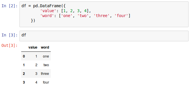
Working With Pandas
A label was added to the rows: an integer incrementing from zero.
Usually that's fine: indexing individual elements is rare anyway. We usually work on entire DataFrames/Series at once.
Working With Pandas
You can read/write entire series with a single operation:
df['double'] = df['value'] * 2
print(df)
print(df[df['value'] % 2 == 0])
value word double 0 1 one 2 1 2 two 4 2 3 three 6 3 4 four 8 value word double 1 2 two 4 3 4 four 8
Note: the labels aren't a position: they are really labels that stay with the rows as they are manipulated.
Working With Pandas
Rows are identified by their label, not their order: that's usually very convenient.
french_words = pd.Series(
    ['trois', 'deux', 'un'],
    index=[2, 1, 0]
)
df['french'] = french_words
print(df)
value word double french 0 1 one 2 un 1 2 two 4 deux 2 3 three 6 trois 3 4 four 8 NaN
Also note: missing values are okay. Represented as not a number
.
Working With Pandas
Like with NumPy arrays, you almost always want to work with DataFrames as a unit, not row-by-row. Another example:
cities = pd.DataFrame(
  [[2463431, 2878.52], [1392609, 5110.21], [5928040, 5905.71]],
  columns=['population', 'area'],
  index=pd.Index(['Vancouver','Calgary','Toronto'], name='city')
)
print(cities)
population area city Vancouver 2463431 2878.52 Calgary 1392609 5110.21 Toronto 5928040 5905.71
Working With Pandas
You can apply Python operators, or methods on a Series, or a NumPy ufunc, or ….
def double_plus(x):
    return 2*x + 1
double_plus = np.vectorize(double_plus, otypes=[np.float64])

cities['density'] = cities['population'] / cities['area']
cities['pop-rank'] = cities['population'].rank(ascending=False)
cities['something'] = double_plus(cities['population'])
print(cities)
population area density pop-rank something city Vancouver 2463431 2878.52 855.797771 2.0 4926863.0 Calgary 1392609 5110.21 272.515024 3.0 2785219.0 Toronto 5928040 5905.71 1003.781086 1.0 11856081.0
Working With Pandas
It's occasionally useful to change the index to a data column, or a data column to the index.
del cities['something']
cities = cities.reset_index()
cities = cities.set_index('pop-rank')
print(cities)
city population area density pop-rank 2.0 Vancouver 2463431 2878.52 855.797771 3.0 Calgary 1392609 5110.21 272.515024 1.0 Toronto 5928040 5905.71 1003.781086