Machine Learning: Classification
CMPT 353
Machine Learning: Classification
Regression is fun, but let's tackle some different problems…
Machine Learning: Classification
With regression, we assumed we were taking input and producing a quantity: what number (continuous value) do we think \(y\) will be (close to) for a particular input?
Many ML problems have a more limited set of outputs. Often the question is more like: which category is this input (mostly likely) part of?
Machine Learning: Classification
These are classification problems. Our outputs will be restricted to the possible classes for our problem. i.e. for \(n\) samples with \(K\) categories, we predict a vector of \(n\) values chosen from \(C_1, C_2,\ldots,C_K\).
Our inputs will stay the same: an \(n\times m\) matrix of numbers (for \(n\) samples and \(m\) features). Or a DataFrame with \(m\) (numeric) columns and \(n\) rows.
Machine Learning: Classification
Some problems that can be seen as classification:
- Is this email spam? Is this credit card charge fraud? (2 categories)
- What (English) word did the user say into the microphone? (≈470k categories *)
- On what day will the first snow fall this winter? (≪365 categories) Or is that regression?
- How many people are in this picture? Who are the people?
Machine Learning: Classification
And ones we will meet in the exercises:
- Given an RGB colour value, what colour word describes it?
- Given weather observations, can you guess what city are we looking at?
Machine Learning: Classification
Broadly, we know this about ML now:

Machine Learning: Classification
There are many ways to model classification. All do the same basic job: train on known data, then make predictions about correct category for other inputs.
model = SomeClassifierModel(…)
model.fit(X_train, y_train)
y_predicted = model.predict(X_valid)
somehow_compare_results(y_valid, y_predicted)
Naïve Bayes
Look at the prediction problem this way: we have an input observation \(\mathbf{x}=[x_1, \dots, x_m]\) and possible output classes \(C_k\). We can ask what the probability of each category is, given the input we saw:
\[P(C_k \mid x_1, \dots, x_m)\,.\]i.e. the probability of \(C_k\) being true
, given that we have the observation \(x_1, \dots, x_m\).
Naïve Bayes
If we can get values \(P(C_k \mid x_1, \dots, x_m)\) for every possible category, then we can look for the category with highest probability and predict it.
That is, we will do maximum likelihood estimation.
Let's look at some details… it's a good example of a machine learning way to look at the world.
Naïve Bayes
You remember everything about conditional probability, right? Nevermind.
What we need right now is Bayes' theorem,
\[P(A\mid B)={P(B\mid A)\frac {P(A)}{P(B)}}\,.\]Naïve Bayes
Some algebra happens. It's very exciting. Then,
\[P(C_{k}\mid x_{1},\dots, x_{m}) = \frac{1}{Z} P(C_{k}) \prod_{i=1}^{m}P(x_{i}\mid C_{k})\,, \]…where \(Z\) is some positive constant. We choose the prediction \(k\) that maximizes this.
Naïve Bayes
Bayes' theorem let us work from \(P(\mathbf{x} \mid C_k)\) to
There are two things in that equation-to-maximize that we need to fill in:
\[\begin{gather*} P(C_{k}) \\ P(x_{i}\mid C_{k}) \mbox{ for each } i \end{gather*}\]Naïve Bayes
P.S. the hidden algebra assumed that \(P(x_{i}\mid C_{k})\) and \(P(x_{j}\mid C_{k})\) are independent. That's the naïve
part of the naïve Bayes classifier
: we are assuming the input features are not related to each other.
Bayesian Classifier
Let's not lose sight of the goal: classify data by learning from known values. Suppose we have points like this with two input features:

Bayesian Classifier
We look at each axis/feature and ask about the distribution of each category.
In statistical terms: we take these as samples and look at the sample distribution.
We will assume normal distributions and calculate \(\overline{x}\) and \(s\) to estimate \(\mu\) and \(\sigma\). That gives us \(P(x_{i}\mid C_{k})\) for each category.
Bayesian Classifier

Bayesian Classifier
Of course, there's a built-in estimator for this. We can ask for the mean and variance of each category in each dimension:
from sklearn.naive_bayes import GaussianNB
model = GaussianNB()
model.fit(X_train, y_train)
print(model.theta_)  # sample means
print(model.sigma_)  # sample variances
[[-1.23392146 -9.46869771]
 [ 1.06460408 -1.47413687]
 [-1.57006349 -3.55600936]]
[[1.57034787 1.67944046]
 [1.38394941 1.5657019 ]
 [1.32418564 1.22885581]]
Bayesian Classifier
Calling model.predict now looks at the (joint) normal distributions and asks which is larger.

Bayesian Classifier
The probability distributions have these values along the \(x=0\) line:

Checking the Classifier
For any classifier, it makes sense to ask about the accuracy: what fraction did the model get right?
y_predicted = model.predict(X_valid)
print(model.score(X_train, y_train))
print(model.score(X_valid, y_valid))
0.944
0.952
Again, the score on the validation data is what we care about most.
Checking the Classifier
Or some more detail. Precision: how many selected were correct. Recall: how many correct were found?
from sklearn.metrics import classification_report
print(classification_report(y_valid, y_predicted))
precision recall f1-score support
0 1.00 1.00 1.00 54
1 0.89 0.94 0.92 35
2 0.94 0.89 0.91 36
avg / total 0.95 0.95 0.95 125
Checking the Classifier
Because the Bayesian classifier has the underlying probability distributions, we can see if the decision was close or not.
X_check = [
    [2, -6], # near the three-way boundary
    [0, -3], # near the red/green (1/2) boundary
]
print(model.predict(X_check))
print(model.predict_proba(X_check))
[1 2]
[[2.92988193e-01 3.98775963e-01 3.08235844e-01]
 [2.61360628e-06 4.44148399e-01 5.55848987e-01]]
Bayesian Priors
We got good results, but we left out one thing we were supposed to know: \(P(C_{k})\), the probability of finding each category (independent of observations).
\[P(C_{k}\mid x_{1},\dots, x_{m}) = \frac{1}{Z} P(C_{k}) \prod_{i=1}^{m}P(x_{i}\mid C_{k})\,, \]Bayesian Priors
To see why it matters, let's look at another data set. There are about a third as many blue (category 0) points as the others. (I counted.)

Bayesian Priors
We can specify a prior to the classifier: what is our belief in the likelihood of each category before we start looking at predictions?
This will be used to weight the categories and adjust the model.
Bayesian Priors
In this case, being honest gets us a nice boost in accuracy.
model = GaussianNB(priors=[1/3, 1/3, 1/3])
model.fit(X_train, y_train)
print(model.score(X_valid, y_valid))
model = GaussianNB(priors=[1/7, 3/7, 3/7]) # == default
model.fit(X_train, y_train)
print(model.score(X_valid, y_valid))
0.8854166666666666
0.921875
Bayesian Priors
The change in decisions is subtle, but apparently makes a difference.

Bayesian Priors
By default, the priors are calculated from the training data distribution, so unless we know more than that, specifying explicitly won't help.
model = GaussianNB()
model.fit(X_train, y_train)
print(model.score(X_valid, y_valid))
0.921875
Bayesian Failures
Remember the assumptions in the Naïve Bayes analysis/model: the components of the input are independent, and we can look at them as normally-distributed.
If those don't hold, we're going to make bad predictions.
Bayesian Failures
For example, these aren't normal in either dimension:

Bayesian Failures
Train/validation split; train; predict. GaussianNB makes these predictions:

Bayesian Failures
The solutions there is probably to pick a different classifier: a Bayesian classifier can't create a decision boundary that will capture this shape.
What about another case, where it looks like we should be able to get somewhere…
Bayesian Failures
These are reasonably-distributed, but the components are not independent (as the naïve Bayesian classifier assumes).

Bayesian Failures
If we just throw GaussianNB at it, nothing good happens.

Bayesian Failures
We could remove the relationship. Because I know (1) how I created the data and (2) arithmetic, I can transform the data (\(x - y \rightarrow x_{new}\)).

Bayesian Failures
We can add this transform to a pipeline and train that.
def de_skew(X):
    X0 = X[:, 0] - X[:, 1]
    X1 = X[:, 1]
    return np.stack([X0, X1], axis=1)

model = make_pipeline(
    FunctionTransformer(de_skew, validate=True),
    GaussianNB()
)
model.fit(X_train, y_train)
Bayesian Failures
That gets some good results:

Bayesian Failures
The lessons:
- You can't just blindly throw an ML tool at data and expect magic.
- Knowing what's happening in your data matters.
- Understanding what the model assumes and how it works will help you use it effectively.
Nearest Neighbours
Let's put another tool in our classification toolbox…
The Naïve Bayesian classifier was simple enough, but maybe we can do something even simpler.
Nearest Neighbours
What if our prediction was just what training point are we closest to?
Nearest Neighbours
That works pretty well, but it looks like we're overfitting the training data.

Nearest Neighbours
Looking at it with the validation data shows the sensitivity to individual training points.

Nearest Neighbours
Instead of looking at the one nearest training point, we could look at \(k\) and have a vote: a \(k\)-nearest neighbours classifier.
e.g. with \(k=5\), we might want to predict a category for point and find that the nearest five training points are green, green, red, green, red. Take the most common and predict green.
Nearest Neighbours
That smooths out some of the overfitting and seems to make fairly reasonable predictions. Same validation data with \(k=5\):

Nearest Neighbours
Of course, it's easy to have scikit-learn do it:
from sklearn.neighbors import KNeighborsClassifier
model = KNeighborsClassifier(n_neighbors=5)
model.fit(X_train, y_train)
print(model.score(X_train, y_train))
print(model.score(X_valid, y_valid))
0.9493333333333334
0.944
… not bad for such a simple technique.
Nearest Neighbours
How do you choose \(k\)?
There's tradeoff. If \(k\) is too small, you'll overfit the training data. If it's too large, you'll underfit reality.
It depends. Experiment.
Nearest Neighbours
kNN can create a complicated boundary shape (both with KNeighborsClassifier(9)):

More Than Points
It's easy to show examples that are 2D points: they make nice figures and are easy to visualize, but they aren't so realistic.
Let's look at some more realistic data: there are lots of example data sets out there for ML experimentation: UCI Machine Learning Repository, KDnuggets dataset list, Kaggle competitions.
More Than Points
Scikit-learn has some data sets built-in.
from sklearn.datasets import load_breast_cancer
bc = load_breast_cancer()
print(bc.data.shape)
print(bc.target.shape, np.unique(bc.target))
print(bc.feature_names)
X = bc.data
y = bc.target
(569, 30)
(569,) [0 1]
['mean radius' 'mean texture' 'mean perimeter' 'mean area'
 'mean smoothness' 'mean compactness' 'mean concavity'
 'mean concave points' 'mean symmetry' 'mean fractal dimension'
 'radius error' 'texture error' 'perimeter error' 'area error'
 'smoothness error' 'compactness error' 'concavity error'
 'concave points error' 'symmetry error' 'fractal dimension error'
 'worst radius' 'worst texture' 'worst perimeter' 'worst area'
 'worst smoothness' 'worst compactness' 'worst concavity'
 'worst concave points' 'worst symmetry' 'worst fractal dimension']
More Than Points
Applying a randomly-chosen classifier does surprisingly well.
model = GaussianNB()
model.fit(X_train, y_train)
print(model.score(X_valid, y_valid))
print(classification_report(y_valid, model.predict(X_valid)))
0.9440559440559441
              precision    recall  f1-score   support

           0       0.94      0.91      0.93        55
           1       0.94      0.97      0.96        88

    accuracy                           0.94       143
   macro avg       0.94      0.94      0.94       143
weighted avg       0.94      0.94      0.94       143
Let's ignore the implications of the 5.6% inaccuracy.
More Than Points
kNN seems to do slightly worse.
model = KNeighborsClassifier(n_neighbors=9)
model.fit(X_train, y_train)
print(model.score(X_valid, y_valid))
0.9230769230769231
More Than Points
But consider the values we're dealing with: mean radius
, texture error
, worst concavity
, …
What scale are those on, and does nearest
make any sense? Is one mean radius
unit comparable to one worst concavity
unit?
More Than Points
The scales are completely different. Measuring nearest
counts mean radius
as much more important than worst concavity
.
bc_df = pd.DataFrame(bc.data, columns=bc.feature_names)
print(bc_df[['mean radius', 'worst concavity']].describe())
mean radius worst concavity count 569.000000 569.000000 mean 14.127292 0.272188 std 3.524049 0.208624 min 6.981000 0.000000 25% 11.700000 0.114500 50% 13.370000 0.226700 75% 15.780000 0.382900 max 28.110000 1.252000
More Than Points
The mean radius
has a range of 6.98 to 28.11, but worst concavity
has a range of only 0 to 1.25 units.

Even a small change in the mean radius
value is going to completely dominate worst concavity
when doing length calculations, so worst concavity
is going to effectively be ignored for nearest-neighbours calculations.
Feature Scaling
At the very least, we can bring the features into a similar range.
This is a common transformation step at the start of a model: scale each feature separately so they have the same size
. That could mean scaling your data so the training data has:
- the smallest value is 0 and the largest is 1.
- the mean is 0 and standard deviation is 1.
- something else that makes sense for your data.
Feature Scaling
There's a transformer for that.
from sklearn.preprocessing import MinMaxScaler, StandardScaler
model = make_pipeline(
    MinMaxScaler(),
    KNeighborsClassifier(n_neighbors=9)
)
model.fit(X_train, y_train)
print(model.score(X_valid, y_valid))
0.958041958041958
Better than plain KNeighborsClassifier or GaussianNB.
Feature Scaling
It's still not obvious that one mean radius (scaled)
should be compared to one worst concavity (scaled)
, but at least the features all contribute to the prediction now.

Will scaling have any effect on the GaussianNB results?
Feature Engineering
Not surprisingly, the kind of X values we have for each training point have a huge effect on what we can learn/predict.
The components of each X value are the features.
A combination of understanding our data and the model can help us be much more successful.
Feature Engineering
We have seen:
- Just use the original features.
- Calculate powers of the original features (
PolynomialFeatures). - Scale features to tidy their min/max (
MinMaxScaler) or mean/stddev (StandardScaler). - Calculate anything else we want/need (
FunctionTransformer).
Feature Engineering
We can design whatever features we think will give the model something to work with. As an example:

Feature Engineering
We could try a kNN model, and it does okay.
model = KNeighborsClassifier(7)
model.fit(X_train, y_train)
print(model.score(X_valid, y_valid))
0.8053097345132744
Feature Engineering
It doesn't have enough training data to really capture what's going on, and overfits the training data.

Feature Engineering
The X values that we have are missing a value that I think is important: how far the point is from \((0,0)\).
We can create a transformer to add that feature…
Feature Engineering
def add_radius(X):
    X0 = X[:, 0]
    X1 = X[:, 1]
    R = np.linalg.norm(X, axis=1) # Euclidean norm
    return np.stack([X0, X1, R], axis=1)

model = make_pipeline(
    FunctionTransformer(add_radius, validate=True),
    GaussianNB()
)
model.fit(X_train, y_train)
print(model.score(X_valid, y_valid))
0.8938053097345132
Feature Engineering
When given the right features, the model can do much better.

Feature Engineering
In Exercise 7 (and 8), the colour data benefits from some work on the features.
It turns out RGB colours aren't particularly well related to human perception. Colour words are all about human perception, and so is the LAB colour space. Or maybe in the HSV colour space, the hue will be a useful feature. Conversion to more semantically meaningful values gets better results.
Feature Engineering
One more example: exercise 8 weather prediction. The problem is to take weather observations (min/max temperature, precipitation, snowfall, snow depth) and predict the city they come from.
I started with 365×5 = 1825 values for each observation (city/year). Problems:
- large data set, requiring lots of processor/memory.
- more features than train+validation data. Hard to learn the many parameters needed.
Feature Engineering
So, I aggregated months together and took the mean of the values. Roughly like:
tmax = tmax.groupby(['city', 'year', 'month']).agg(np.mean)
tmax = pd.pivot_table(tmax, index=['city', 'year'], …)
That gives 12×5 = 60 features that are much easier to work with.
This aggregation was chosen because I understand the data. Averaging values values in each month
makes sense and will smooth out noisy weather changes; averaging first of every month
doesn't.
Decision Trees
All of our classification techniques are essentially fancy if statements, where the model decided on the condition for us.
if ???:
    return 'red'
elif ???
    return 'orange'
⋮
Decision Trees
For a problem like digit recognition, maybe it could be thought of like this:
def recognize_digit(img):
    if img[4,8] < 30 and img[32,18] > 10 and …:
        return '1'
    elif img[27,0] > 100 and img[15,86] == img[45,6] and …:
        return '2'
    ⋮
Once again, thinking this way can lead us to a reasonable classifier algorithm.
Decision Trees
Here's the idea: we have a bunch of features, but pick one. Look at it and ask if the value is low or high.
Take the training data where the value is low. Recursively do the same: pick some other feature, examine its value, and branch.
Same for the else
case where the value is high.
This would effectively build a big nested if/else structure. At the end of each branch, make a prediction.
Decision Trees
Let's return to this example →
We could make some very simple decisions. If the \(y\) is small, predict blue. Else if \(x\) is small predict red, else green.
Decision Trees
As our decisions get more complex, it's much easier to think of it as a tree than an if/else structure.
A decision tree.

Decision Trees
Once again, Scikit-Learn will do the hard work.
from sklearn.tree import DecisionTreeClassifier
model = DecisionTreeClassifier(max_depth=2)
model.fit(X_train, y_train)
print(model.score(X_train, y_train))
print(model.score(X_valid, y_valid))
0.9386666666666666
0.912
Decision Trees
From that strategy, we get these decision boundaries:

Decision Trees
Scikit-learn will also visualize the decision tree for us:

Decision Trees
We can let the tree be a little more complex, to make more complex predictions.
model = DecisionTreeClassifier(max_depth=4)
model.fit(X_train, y_train)
print(model.score(X_train, y_train))
print(model.score(X_valid, y_valid))
0.968
0.944
Decision Trees
The decision boundaries:

Decision Trees
The tree:

Decision Trees
As with other algorithms, more complexity in the model means more freedom in decisions, but also possibly over-fitting the training data.
model = DecisionTreeClassifier(max_depth=15)
model.fit(X_train, y_train)
print(model.score(X_train, y_train))
print(model.score(X_valid, y_valid))
1.0
0.912
More loss between training validation scores suggests over-fitting. Also, validation score decreased.
Decision Trees
The decision boundaries tell the same story:

Decision Trees

Decisions
In those examples, our trees all started by looking at \(y<-6.343\). Why that decision? How is the decision tree built?
The details are complex, but the idea is…
Decisions
We need some way to evaluate if a split is good. Common choices: Gini impurity and information gain.
Both are a measure of how pure
a branch is. If we can split so that 100% of values on each side are in one category, then that's good. If we split so that every outsome is equally likely on each side, that's bad. Create the decision that maximizes goodness
.
Decisions
Gini impurity does this measuring the probability of getting a label wrong if we predict using frequency of training points down either side. We minimize the probability of error.
Information gain measures the information entropy of either branch. We want to minimize entropy (and thus maximize information gain).
Decisions
Either method seems to produce similar trees. In either case, we create a decision, and then recurse until we have to stop.
Deciding how to stop building the tree is more interesting in a practical sense…
Limiting the Tree
We saw that a too-complex tree will over-fit the training data. The defaults for DecisionTreeClassifier have few limits on the tree size, so will over-fit unless you do something about it.
When I built the example trees, I simply limited the tree height. In this case, make at most 4 comparisons before the model must make its prediction.
model = DecisionTreeClassifier(max_depth=4)
Limiting the Tree
Another option: how many nodes must be on a branch before it's too small to split?
model = DecisionTreeClassifier(min_samples_split=30)
Or how much support do we need for a leaf?
model = DecisionTreeClassifier(min_samples_leaf=10)
Or we can combine those in any way we like…
Limiting the Tree
model=DecisionTreeClassifier(max_depth=6, min_samples_leaf=4)

Ensembles
It can sometimes be hard to balance the complexity of the classifier with over-fitting. Sometimes, we'll find that no single classifier will do a great job on the problem.
It can be easy to produce a classifer that makes predictions better than chance, but still not great. It turns out that's still useful…
Ensembles
It's often useful to have many simple classifiers, with some differences in their construction/training so they produce different results, and let them vote: an ensemble.
An ensemble can often produce good results, even though the individual classifiers are quite bad.
Ensembles
Usually, all of the models will be of the same type, but they don't have to be. A VotingClassifier will let you combine any collection of models you want, train them together, and vote on predictions.
model = VotingClassifier([
    ('nb', GaussianNB()),
    ('knn', KNeighborsClassifier(5)),
    ('svm', SVC(kernel='linear', C=0.1)),
    ('tree1', DecisionTreeClassifier(max_depth=4)),
    ('tree2', DecisionTreeClassifier(min_samples_leaf=10)),
])
model.fit(X_train, y_train)
print(model.score(X_train, y_train))
print(model.score(X_valid, y_valid))
Random Forests
An ensemble of decision trees is often a good model: one tree seems to often be either too simple or over-fit. Many trees in an ensemble often do better than a single tree.
We'll introduce some randomness into the construction of the trees so they are different, put many (possibly dozens or hundreds) of them togther, and have a vote. A random forest.
Random Forests
Each decision tree will be constructed as before, but…
- individual trees will likely be simpler (lower max depth, fewer leaves, etc);
- when training, use only a sample of the training data (chosen randomly with replacement, a bootstrap sample);
- for each decision, consider only a random subset of the features.
… and repeat many times.
Random Forests
When constructing a random forest, we get the same options as a decision tree about the tree shape, plus the number of estimators (and some other choices about the randomness of the construction).
from sklearn.ensemble import RandomForestClassifier
model = RandomForestClassifier(n_estimators=100,
        max_depth=3, min_samples_leaf=10)
model.fit(X_train, y_train)
print(model.score(X_train, y_train))
print(model.score(X_valid, y_valid))
0.9653333333333334
0.92
Random Forests
We get a reasonable-looking decision boundary.

Random Forests
A few of the decision trees from the forest:


Random Forests
None of the individual trees make great decisions, but together they do.


Random Forests
The voting among trees can also help with over-fitting: since each was trained with a subset of the data, it's less of a problem.
Let's try some data from make_moons. We can say very little about tree size but still get good results:
model = RandomForestClassifier(n_estimators=400, max_depth=7)
model.fit(X_train, y_train)
print(model.score(X_train, y_train))
print(model.score(X_valid, y_valid))
1.0
1.0
Random Forests
There is still maybe some over-fitting (actually under-training), but it's not affecting the scores.

Boosting
We can push the idea of ensembles a little further: instead of creating an independent collection of estimators, maybe we can design them to work together.
To get this to work, we'll introduce the idea of weighting the training data. Each training point gets a weight. When calculating the score, use the weight to decide how important
it was that each point is predicted right/wrong.
Boosting
The idea: start each training point with equal weights. Train a classifier (decision tree).
Look at the forest up to this point: what training points are classified incorrectly? Increase their weights. Decrease weights where predictions are correct.
Repeat until you have the number of trees you want.
The effect: each subsequent tree concentrates
on the examples missed previously.
Boosting
The AdaBoostClassifier and GradientBoostingClassifier both implement boosted tree algorithms with different details.
Empirically, boosted trees seem to be an excellent way to attack many ML problems: they are often a good first choice for a new problem.
Boosting
For example, on the breast cancer data set:
from sklearn.ensemble import GradientBoostingClassifier
model = GradientBoostingClassifier(n_estimators=50,
        max_depth=2, min_samples_leaf=0.1)
model.fit(X_train, y_train)
print(model.score(X_train, y_train))
print(model.score(X_valid, y_valid))
0.9976525821596244
0.965034965034965
That's the best validation score we have seen in our attempts on this data.
Higher Dimensions
The breast cancer data set had 30 features. The Exercise 8 weather data has 60. Those are manageable.
But it's easy to end up with lots more input features than that, particularly with images.
Higher Dimensions
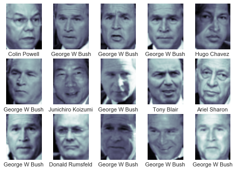
Another built-in data source: images of famous people, labelled with their names from the Labelled Faces in the Wild project.
from sklearn.datasets import fetch_lfw_people
faces = fetch_lfw_people(min_faces_per_person=60, resize=1.0)
print(faces.target_names)
print(faces.images.shape)
['Ariel Sharon' 'Colin Powell' 'Donald Rumsfeld' 'George W Bush'
 'Gerhard Schroeder' 'Hugo Chavez' 'Junichiro Koizumi' 'Tony Blair']
(1348, 125, 94)
i.e. 1348 images, each 125×94 = 11750 pixels (greyscale).
Higher Dimensions
The goal is to train a model to take the image and predict the name. Suddenly we have 11750 input features on a toy-sized image task.
Higher Dimensions
A simple classifier does better that I would have expected.
X_train, X_valid, y_train, y_valid = \
        train_test_split(faces.data, faces.target)
model = SVC(kernel='linear', C=2.0)
model.fit(X_train, y_train)
print(model.score(X_valid, y_valid))
0.8189910979228486
Higher Dimensions
This model takes ≈8 seconds to train. Running time depends on the number of features.
[Naïve Bayes, kNN, and a random forest are much faster, but much worse results: scores 0.48, 0.54, 0.55, respectively.]
Higher Dimensions
The SVM algorithm's running time depends on the number of features: we need to somehow decrease the number of input features.
They're probably not all important: is pixel (0, 0) really important to the prediction? Aren't some pixels very highly correlated?
Maybe we can do something about that…
Higher Dimensions
One option: scale down the images.
Scaling to 50% of the original size trains an SVM in ≈1.8 seconds with almost exactly the same accuracy.
Once again: understanding your data is better than all the algorithms in the world. But that doesn't motivate the next topic…
PCA
We would like to decrease the number of dimensions, but keep the information that matters.
The solution is going to be Principal Component Analysis (PCA)…
PCA
Consider this two-dimensional data.
How two-dimensional is it really? Most of what's happening is along the diagonal. It's almost one-dimensional (but it's not the existing \(x\) or \(y\)).

PCA
Principal component analysis finds the directions where most of the interesting stuff is happening
The idea behind the calculation… Find the vector along which the data has the maximum variance: that's the first principal component. Collapse the data along that vector. Recurse until you're out of dimensions.
[Actually, there's a pile of linear algebra, which I'm going to ignore.]
PCA
As usual, scikit-learn does the hard work…
from sklearn.decomposition import PCA
pca = PCA(2)
pca.fit(X)
print(pca.components_)
print(pca.explained_variance_ratio_)
[[-0.80111387 -0.59851197]
 [-0.59851197  0.80111387]]
[ 0.99027873  0.00972127]
Output here: the components, in order of decreasing variance; the fraction of the variance along each.
PCA
Graphically, the principal components are:

99% of the variance is in the red direction; 1% purple.
PCA
The PCA transformer can make those two things the new axes of the data.
X_pca = pca.transform(X)

PCA
Assuming we start with \(m\) dimensional data, and look for \(m\) principal components, we're not really losing anything (except a little floating point error).
X_after_pca = pca.inverse_transform(pca.transform(X))
print(np.abs(X_after_pca - X).max())
8.881784197e-16
PCA
Sometimes, PCA can help you get a better idea what's going on with your data. On the breast cancer data:
scale = StandardScaler()
pca = PCA(2)
X_pca = pca.fit_transform(scale.fit_transform(X))

PCA
Obviously, some of the data in the original 30 dimensions is being lost, but we can kind of see how a model can separate the two classes.
PCA
Probably the most useful PCA application for us: dimensionality reduction.
The face images had 11750 dimensional features. Getting rid of many of them doesn't lose much.
model = make_pipeline(
    PCA(250),
    SVC(kernel='linear', C=2.0)
)
model.fit(X_train, y_train)
print(model.score(X_valid, y_valid))
0.8130563798219584
PCA
Comparison: [Notebook that does the timing]
| Method | Accuracy | Time |
|---|---|---|
| full data SVM | 0.834 | 7.8 s |
| PCA → SVM | 0.825 | 1.5 s |
| scale 50% → SVM | 0.825 | 1.8 s |
| scale → PCA → SVM | 0.816 | 0.5 s |
Of course, results will vary for different problems/data.
PCA
What did going from 11750 to 250 dimensions lose us?
pca = model.named_steps['pca']
img_orig = X_valid[0]
img_trans = pca.inverse_transform(pca.transform([img_orig]))[0]

PCA
PCA can be a useful way to look at your data.
Sometimes, it's the only way to be able to get anywhere if the large number of dimensions is the problem.
Imbalanced Data
If you have training data where some categories don't have many training points, it can be very hard to train a model well.
e.g. If you have 1000 training points, 990 in class A and only 10 in class B, the model can get an accuracy score of 0.99 by always predicting A. Good score; useless model.
Imbalanced Data
Let's try an example: Seismic Bumps
data set. Interesting problem, but seismic bumps are rare.
print(data['class'].value_counts())
class
0    2414
1     170
6.6% of the data is in class 1 (seismic bump). That's actually not too imbalanced, but…
Imbalanced Data
First we need to make sense of the data: there are several non-numeric fields that won't work with Scikit-Learn.
Some are seismic hazard assessment
values described as:
a - lack of hazard, b - low hazard, c - high hazard, d - danger state
I'm going to call those ordinal and make then numeric by mapping to numbers 0–3.
Imbalanced Data
There is also a categorical feature: shift
is either 'N' or 'W' to describe what was happening that day.
To make the categorical data numeric, I am going to one-hot encode it: each category will have a feature column that is 1 in we're in that category, and 0 otherwise. i.e. we will have a binary column is in category N
and another is in category W
.
Imbalanced Data
The seismic hazard assessment
columns can be handled with a function transformer that does some Pandas work to map the letters to numbers:
assessment_map = {b'a': 0, b'b': 1, b'c': 2, b'd': 3}
def seismic_features(data):
    data['seismic'] = data['seismic'].map(assessment_map)
    data['seismoacoustic'] = data['seismoacoustic'].map(assessment_map)
    data['ghazard'] = data['ghazard'].map(assessment_map)
    return data
Imbalanced Data
The one-hot encoding can be done with OneHotEncoder on the 'shift' column. To send different columns through different transformers, I found ColumnTransformer:
model = make_pipeline(
    ColumnTransformer([
        ('assements', FunctionTransformer(seismic_features, validate=False),
            ['seismic', 'seismoacoustic', 'ghazard']),
        ('onehot', OneHotEncoder(), ['shift']),
    ], remainder='passthrough'),
    SimpleImputer(strategy='mean'),
    GradientBoostingClassifier(n_estimators=50, max_depth=3, min_samples_leaf=0.1)
)
Imbalanced Data
With a randomly-chosen model, we get good scores:
0.9226006191950464
0.9380804953560371
Imbalanced Data
But the classification report tells the story more clearly:
0.9380804953560371
              precision    recall  f1-score   support

           0       0.92      1.00      0.96       596
           1       0.00      0.00      0.00        50

    accuracy                           0.92       646
   macro avg       0.46      0.50      0.48       646
The model is never predicting category 1.
Imbalanced Data
Or the confusion matrix tells the same story.
ConfusionMatrixDisplay.from_estimator(model, X_valid, y_valid)

Imbalanced Data
There are several ways to deal with imbalanced data: balance the data set, use something more fair than the accuracy score, adjust the model so it can make more subtle decisions, generate more data.
Imbalanced Data
I'm going to re-balance the data: keep the rare data, and sample an equal amount of the common class.
bump = data[data['class'] == 1]
nobump = data[data['class'] == 0].sample(n=bump.shape[0])
balanced_data = pd.concat([bump, nobump])
i.e. keep all of the category 1 data, and randomly sample an equal number from the other class.
Imbalanced Data
We lose some accuracy, but have a much more useful model.
0.7411764705882353
0.8549019607843137
              precision    recall  f1-score   support

           0       0.73      0.76      0.74        42
           1       0.76      0.72      0.74        43

    accuracy                           0.74        85
   macro avg       0.74      0.74      0.74        85
weighted avg       0.74      0.74      0.74        85
Imbalanced Data
Be on the lookout for imbalanced data in your project (or other ML work). Remember to deal with non-numeric data appropriately.
Motivating Neural Nets
The classifiers we have talked about (Naïve Bayes, kNN, trees) are useful. Each looks at the training data a different way and trains itself to predict on future points. Big and hard problems can often be attacked with neural network-based techniques…
Motivating Neural Nets
Let's come at the classification
problem another way…
We have been working with training/validation data called \(\mathbf{X}\) (in code, X or X_train or similar). Each observation is a row in that matrix, with some inputs \(\vec{x} = (x_1,x_2,\ldots,x_m)\).
Motivating Neural Nets
For the various predictions we could make, the features matter different amounts. Maybe can quantify how much each feature's value predicts category \(C_i\).
We'll assign a weight to each category and feature.
Motivating Neural Nets
Let's return to this data →
I made up this calculation for some magic number:
\[ -28.6 - 1.2x_1- 4.9x_2\,. \]If that number is large, I'll take that as evidence for being in category 0 (blue).
[Note: I'm relabeling \((x_0, x_1)\) as \((x_1, x_2)\), because we'll want that later.]
Motivating Neural Nets
I also made up similar magic calculations for categories 1 and 2:
\[\begin{align*} \mathit{magic}_0 &= -28.6 - 1.2x_1 - 4.9x_2 \\ \mathit{magic}_1 &= 17.2 + 1.9x_1 + 3.2x_2 \\ \mathit{magic}_2 &= 13.2 + 0.04x_1 + 1.9x_2 \\ \end{align*}\]Whichever one is largest, I predict the corresponding category.
Motivating Neural Nets
My model with magic calculations does well.

Motivating Neural Nets
I have even more faith in my magic numbers: I will scale them so each prediction has a sum of one and interpret them as probabilities. [Scaling of each row will be done by the softmax function.]
X_check = [
    [2, -6], # near the three-way boundary
    [0, -3], # near the red/green (1/2) boundary
]
model = FunnyMagicModel()
print(model.predict_proba(X_check))
[[1.57669463e-02 4.72442358e-01 5.11790696e-01]
 [2.41440836e-10 5.24979187e-01 4.75020812e-01]]
Perceptrons
So what just happened? I invented a perceptron.
- Add a column of 1s to (the left of) our \(\mathbf{X}\) matrix. Call it the bias.
- Call the magic numbers weights and put them in a matrix \(\mathbf{W}\).
- Call softmax our activation function, \(f\).
Then our calculation was:
\[ f(\mathbf{W} \cdot \mathbf{X}^{\mathrm{T}}) \]Perceptrons
Or if you'd like it to be more visual, for a particular observation \((x_1,x_2)\), we did:

Perceptrons
Of course, we don't have to guess the weight matrix.
from sklearn.neural_network import MLPClassifier
model = MLPClassifier(solver='lbfgs', hidden_layer_sizes=())
model.fit(X_train, y_train)
print(model.coefs_[0])
print(model.intercepts_[0])
print(model.score(X_valid, y_valid))
[[-1.17782848  1.93625709  0.04458776]
 [-4.85534988  3.21374237  1.89215087]]
[-28.64983462  17.17502741  13.21223349]
0.936
Perceptrons
A perceptron does a reasonable job on simple cases, but we're not interested in simple cases…
Neural Networks
The idea behind a perceptron is good: take inputs, weight them somehow, have an activation function to normalize the results. Do some magic to learn the weights from training data.
But, it doesn't allow enough flexibility in the way predictions are made.
Neural Networks
We can do the same thing, but more. Add extra layers of computation that let more complex decision be made. Call the result a neural network.
Neural Networks
An example. Each edge has its own weight. Each node represents a sum of weighted inputs and an activation function.

Neural Networks
The middle layers don't have any semantic meaning: they let the arithmetic create good decisions.
The softmax activation function doesn't make sense for the middle layers. Common choices: logistic/sigmoid, tanh, rectifier. All do some kind of scale into a reasonable range
operation.
Neural Networks
Here's a scikit-learn way to implement that neural network.
model = MLPClassifier(solver='lbfgs',
    hidden_layer_sizes=(4,3), activation='logistic')
model.fit(X_train, y_train)
print(model.score(X_valid, y_valid))
0.936
Neural Networks

Neural Networks
In this (toy sized) example, we have 39 weights to figure out.
That can't be done analytically. The model must guess some initial weights, then use the training data to improve them until they converge on good
values.
Neural Networks
A couple of results of that…
Training a neural network needs a lot of training data. There is a lot of freedom in the weights, so a lot of examples are needed to get them all trained reasonably.
e.g. In that example (with 375 training points) there isn't really enough to train the weights: there's a lot of randomness to the decision boundary and score. [nn.py, plot_decision.py]
Neural Networks
Training a neural net is very computationally expensive: modern CPUs aren't up to the task. Luckily, the linear algebra invovled in backpropagation is the kind of thing GPUs are good at.
Here, we have to leave scikit-learn behind: it's good for small example neural networks, but not at the realistic scale in modern machine learning.
Neural Networks
There are other toolkits for neural nets that are a lot more capable: Keras, Caffe, PyTorch. Lower-level but neural nets are one thing they can do: Tensorflow, Theano.
These will use your (CUDA-capable NVIDIA, or possibly other OpenCL-capable) GPU if set up properly. CPU if not.
Neural Networks
We need our targets in the form the neural net expects: probabilities of each output. In our example with three categories, that means:
0 → [1, 0, 0]
1 → [0, 1, 0]
2 → [0, 0, 1]
Scikit-learn can do that (and so can other tools):
from sklearn.preprocessing import LabelBinarizer
binarizer = LabelBinarizer()
y = binarizer.fit_transform(y)
Neural Networks
The same model spelled with Keras:
from keras.models import Sequential
from keras.layers.core import Dense, Activation

model = Sequential()
model.add(Dense(4, input_shape=(2,)))
model.add(Activation('sigmoid'))
model.add(Dense(3))
model.add(Activation('sigmoid'))
model.add(Dense(3))
model.add(Activation('softmax'))

model.compile(loss='categorical_crossentropy',
        optimizer='sgd', metrics=['accuracy'])
Neural Networks
Fitting, scoring, and predicting are spelled differently than scikit-learn, but the basic ideas are the same:
model.fit(X_train, y_train, epochs=2000, batch_size=75, verbose=0)
print(model.evaluate(X_valid, y_valid)[1])

y_probab = model.predict(X_valid)
y_predict = model.predict_classes(X_valid)
print(y_probab[:4])
print(y_predict[:4])
0.903999991417
[[ 0.01135819  0.95259881  0.03604292]
 [ 0.01208871  0.95006722  0.03784406]
 [ 0.44920909  0.03528297  0.51550788]
 [ 0.49855995  0.02473667  0.47670344]]
[1 1 2 0]
Neural Networks
The amount of data needed to train a neural network can be a deal-breaker. If a right-sized neural network would need 10000 points to train it properly, it's useless if you have 1000 and no way to get more.
Thus Naïve Bayes, kNN, trees, forests still have their place. They might not be the cutting edge, but are (in general) workable in simpler cases, when you have smaller training sets.
Neural Networks
Some links if you want more:
- But what is a Neural Network?, Gradient descent, how neural networks learn, and What is backpropagation and what is it actually doing? from 3Blue1Brown.
- Neural Networks and Deep Learning, online book/course.
- fast.ai, free neural network MOOC.
Deep Learning
It turns out that those middle layers in the network let interesting things happen.
If your neural network has lots of layers, call it deep learning.
Deep Learning
More layers give more complexity, and more parameters make everything more flexible. The predictions that can be made are astonishing (if you use the complexity well).
GPU power makes training large networks conceivable.
How large?
Deep Learning

An overview of the shape of GoogLeNet Figure 2 from Szegedy et al, Going Deeper with Convolutions, 2014., which was designed for computer vision problems. →
Each box there is a layer, not a single node. The paper says there are ≈6.8M parameters.
Deep Learning
Andrew Ng's estimation of the state-of-the-art:
Pretty much anything that a normal person can do in <1 sec, we can now automate with AI. Andrew Ng, @AndrewYNg, Oct 2016.
At this point, I feel like we're leaving data science
behind. Let's return…