How Spark Calculates
CMPT 353
How Spark Calculates
Some terminology…
The program that you write is the driver. If you print or create variables or do general Python things: that's the driver process.
The data in the DataFrames is managed in one or more executor processes (or threads). They take instructions from the driver about what to do with the DataFrames: perform the calculations, write the output, etc.
How Spark Calculates
When running locally, this all happens in one process. Processor capable of \(n\) concurrent threads → one driver and \(n\) executor threads.
On the cluster, the driver runs on the gateway (the way we're submitting jobs, anyway). YARN starts executors on the cluster nodes.
How Spark Calculates
Any operation on a DataFrame (or RDD, which we'll see later) is done by having executors do work on its partitions. Within a partition, a task is sequential.
The parallelism is controlled by the way the data is partitioned.
How Spark Calculates
If we have 1000 executors and 2 partitions in a DataFrame, 998 executors will be sitting idle.
If we have two executors and two partitions, both will be used. But, if one partition is much bigger than the other, one executor will finish first and then sit idle.
Lesson: the way your data is partitioned matters a lot.
How Spark Calculates
The right
number of partitions depends on the task and size of the DataFrame.
In general, you want (at least) a few times the number of executors: that way one slow executor or large partition won't slow things too much.
There is some overhead to managing the partitions: having too many is expensive.
How Spark Calculates
If I had to give generic advice: a few times as many partitions as cores. My usual default is 10× the number of cores I think I have available.
For small data sets: fewer (even one) is probably fine, but then why use Spark?
For truly big data sets, more might make sense. (Sometimes, just so you can see the progress bar move and know things are happening.)
How Spark Calculates
But the only way we have had to control partitions so far is the structure of the input files: one file became one partition (in every case we've seen).
It's easy to get into trouble right away.
e.g. the Reddit Comment Corpus has comments grouped by month: relatively few files (≈200), and very different sizes (RC_2007-01.bz2 is 7.5 MB, RC_2023-01.zst is 32 GB).
Controlling Partitions
We need more control over partitions in our DataFrames.
Honestly, often easiest: split the input files into something that makes sense before even putting them into HDFS.
Controlling Partitions
There are a few operations where you can explicitly ask for a number of partitions:
int_range = spark.range(100000, numPartitions=6)
int_range.show(5)
print(int_range.rdd.getNumPartitions())
print(partition_sizes(int_range)) # I wrote partition_sizes: nonstandard.
+---+
| id|
+---+
|  0|
|  1|
|  2|
|  3|
|  4|
+---+
only showing top 5 rows

6
[16666, 16667, 16667, 16666, 16667, 16667]
Controlling Partitions
There are some where there's a default of 200. (We'll cover later: shuffle operations
.)
values = int_range.withColumn('mod', int_range['id'] % 3)
counts = values.groupBy('mod').count()
counts.show()
print(counts.rdd.getNumPartitions())
+---+-----+
|mod|count|
+---+-----+
|  0|33334|
|  1|33333|
|  2|33333|
+---+-----+

200
So… 197 empty partitions, and three of size one?
Controlling Partitions
But mostly, we are working with whatever is implied by the input files. If that's not sensible, we have to fix it.
There are a couple of methods that will rearrange the partitions of a DataFrame…
Controlling Partitions
If the problem is too many partitions, the .coalesce(n) can concatenate some of them together.
It might not do quite what you expect, but it will lower the many-partitions overhead if you have it.
Controlling Partitions
I created an oddly-partitioned DataFrame and coalesced to see what happens:
print(partition_sizes(lumpy_df))
print(partition_sizes(lumpy_df.coalesce(4)))
print(partition_sizes(lumpy_df.coalesce(2)))
[0, 300, 150, 0, 0, 220]
[0, 450, 0, 220]
[300, 370]
Controlling Partitions
After the .groupBy(), we had a situation like this, where .coalesce() helps a lot:
print(partition_sizes(after_groupby))
print(partition_sizes(after_groupby.coalesce(3)))
print(partition_sizes(after_groupby.coalesce(1)))
[0, 0, 1, 0, 1, 0, 0, 0, 0, 0, 0, 0, 0, 0, 0, 0, 0, 0, 1, 0]
[2, 0, 1]
[3]
Controlling Partitions
It can clean up your output if you know you have a small number of rows. Produces one output file (with 670 lines in the example, which is reasonable):
# <1000 rows remain after .groupBy()
lumpy_df.coalesce(1).write.json(…)
Controlling Partitions
If you really need a DataFrame's partitions rearranged, the .repartition(n) method does it, but it's more expensive.
print(partition_sizes(lumpy_df.coalesce(4)))
print(partition_sizes(lumpy_df.repartition(4)))
[0, 220, 450, 0]
[168, 167, 167, 168]
Is it worth it? It depends what else is going to be done with that data.
Controlling Partitions
Course rule: if you explicitly decrease the partitions of a DataFrame (or RDD) (with .coalesce or .repartition), you must include a comment justifying why it is a safe thing to do. If not: mark penalty.
You should say something about an upper-bound on the data size. Not the provided sample data sets: all possible inputs.
Controlling Partitions
For example:
weather_data.groupBy('year').count().coalesce(1)
# data provided for 10 years
weather_data.groupBy('year').count().coalesce(1)
# weather data has been recorded for <200 years
weather_data.groupBy('year').count().coalesce(1)
# approx_count_distinct on full data shows 1.2M subreddits
reddit_comments.groupBy('subreddit').count().coalesce(100)
# assignment indicates that 10 partitions is safe
reddit_comments.groupBy('subreddit').count().repartition(10)
# complete data is ~10M rows but partitioned funny
spark.read.json(in_dir).repartition(1000).write.parquet(out)
Controlling Partitions
How many rows do you want in each partition? It depends.
How many total rows in the DataFrame? How many executors? What calculation is going to happen? How much processor and memory will it need?
df.select(df['x'] + 1) # big partitions fine
df.select(find_polynomial_roots(…)) # more caution needed?
Shuffle Operations
I usually think of a DataFrame as a list-like thing (left). We know it's more correctly a collection of partitions (right). [Pictured with 3 integer columns.]

Shuffle Operations
But remember that the partitions might be stored on different physical machines, with a network in the middle. This might be more accurate. * *

Shuffle Operations
If we want to repartition this DataFrame, info needs to be exchanged over the network. That could be slow if it was a big DataFrame.
Shuffle Operations
Any Spark operation that rearranges data among partitions is a shuffle operation. Obviously .repartition() is one.
We also mentioned .sort(): to get everything sorted, the smallest values have to be moved into the first partition, and so on.
Also .groupBy() (more soon).
Shuffle Operations
Any time you do a shuffle operation, you should give a little thought to what you just asked for.
Is the data a reasonable size to move around? Can you accomplish the same thing without shuffling?
Shuffle Operations
The opposite is a pipeline operation: anything where the partitions can be handled completely independently. (Even better: individual rows handled independently.) Most DataFrame operations are in this category.
e.g. .select(), .filter(), .withColumn(), .drop(), .sample(), ….
Grouping Data
We have seen the .groupBy() method a couple of times, but it deserves some explanation.
The idea: you take all rows with the given columns the same, and do some aggregation over those values.
Grouping Data
An artificial example to work with:
int_range = spark.range(10000, numPartitions=6)
values = int_range.select(
    (int_range['id'] % 3).alias('mod'),
    (functions.length(int_range['id'].astype(types.StringType()))).alias('num_digits'),
    int_range['id'],
    functions.sin(int_range['id']).alias('sin')
)
values.show(6)
+---+----------+---+-------------------+
|mod|num_digits| id|                sin|
+---+----------+---+-------------------+
|  0|         1|  0|                0.0|
|  1|         1|  1| 0.8414709848078965|
|  2|         1|  2| 0.9092974268256817|
|  0|         1|  3| 0.1411200080598672|
|  1|         1|  4|-0.7568024953079282|
|  2|         1|  5|-0.9589242746631385|
+---+----------+---+-------------------+
only showing top 6 rows
Grouping Data
You can group by whatever column(s) you want, and aggregate a few different ways.
groups = values.groupBy('mod') # a GroupedData obj, not a DF
result = groups.agg({'id': 'count', 'sin': 'sum'})
result = groups.agg(functions.count(values['id']),
                    functions.sum(values['sin']))
result.show() # results are the same from either of the above.
+---+---------+------------------+
|mod|count(id)|          sum(sin)|
+---+---------+------------------+
|  0|     3334|0.3808604635953807|
|  1|     3333|0.6264613886425877|
|  2|     3333|0.9321835584427463|
+---+---------+------------------+
Grouping Data
Multiple-column grouping:
groups = values.groupBy('mod', 'num_digits')
result = groups.agg(functions.avg(values['id']),
                    functions.max(values['sin']))
result.sort('mod', 'num_digits').show()
+---+----------+-------+------------------+
|mod|num_digits|avg(id)|          max(sin)|
+---+----------+-------+------------------+
|  0|         1|    4.5|0.4121184852417566|
|  0|         2|   55.5|0.9999118601072672|
|  0|         3|  550.5| 0.999990471552965|
|  0|         4| 5500.5|0.9999933680737474|
|  1|         1|    4.0|0.8414709848078965|
|  1|         2|   53.5|0.9928726480845371|
|  1|         3|  548.5|0.9999122598719259|
|  1|         4| 5498.5|0.9999931466878679|
|  2|         1|    5.0|0.9893582466233818|
|  2|         2|   54.5|0.9995201585807313|
|  2|         3|  549.5|0.9999110578521441|
|  2|         4| 5499.5|0.9999935858249229|
+---+----------+-------+------------------+
Execution Plans
Grouping is a shuffle operation, but not as bad as some. To see why, we can ask for the execution plan Spark has for a DataFrame:
result.explain()
== Physical Plan ==
*(2) HashAggregate(keys=[mod#90L, num_digits#91], functions=[avg(id#88L), max(sin#92)])
+- Exchange hashpartitioning(mod#90L, num_digits#91, 200)
   +- *(1) HashAggregate(keys=[mod#90L, num_digits#91], functions=[partial_avg(id#88L), partial_max(sin#92)])
      +- *(1) Project [(id#88L % 3) AS mod#90L, length(cast(id#88L as string)) AS num_digits#91, id#88L, SIN(cast(id#88L as double)) AS sin#92]
         +- *(1) Range (0, 10000, step=1, splits=6)
Execution Plans
== Physical Plan ==
*(2) HashAggregate(keys=[mod#90L, num_digits#91], functions=[avg(id#88L), max(sin#92)])
+- Exchange hashpartitioning(mod#90L, num_digits#91, 200)
   +- *(1) HashAggregate(keys=[mod#90L, num_digits#91], functions=[partial_avg(id#88L), partial_max(sin#92)])
      +- *(1) Project [(id#88L % 3) AS mod#90L, length(cast(id#88L as string)) AS num_digits#91, id#88L, SIN(cast(id#88L as double)) AS sin#92]
         +- *(1) Range (0, 10000, step=1, splits=6)
What we did to create the result DataFrame: range; .select(…); .groupBy('mod','num_digits'); .agg(avg, max).
Even though that happened across several DataFrame objects in my code, it all became the plan for computing result.
Execution Plans
The relevant part for the .groupBy() and .agg():
*(2) HashAggregate(keys=[mod#90L, num_digits#91], functions=[avg(id#88L), max(sin#92)])
+- Exchange hashpartitioning(mod#90L, num_digits#91, 200)
   +- *(1) HashAggregate(keys=[mod#90L, num_digits#91], functions=[partial_avg(id#88L), partial_max(sin#92)])
It starts by doing
and partial_avg
, which are the per-partition aggregations. Then it partial_maxexchanges
(shuffles) and finishes the
and avg
.max
Execution Plans
*(2) HashAggregate(keys=[mod#90L, num_digits#91], functions=[avg(id#88L), max(sin#92)])
+- Exchange hashpartitioning(mod#90L, num_digits#91, 200)
   +- *(1) HashAggregate(keys=[mod#90L, num_digits#91], functions=[partial_avg(id#88L), partial_max(sin#92)])
Result: if we started with billions of rows, but grouped by 10 unique values, then only 10 rows from each partition have to be shuffled.
That's a lot better than the shuffle from a .sort() or .repartition(). Spark has been clever on our behalf.
Execution Plans
Compare the plans for a .repartition() or .sort():
values.repartition(100).explain()
values.sort('sin').explain()
== Physical Plan ==
Exchange RoundRobinPartitioning(100)
+- *(1) Project [(id#88L % 3) AS mod#90L, length(cast(id#88L as string)) AS num_digits#91, id#88L, SIN(cast(id#88L as double)) AS sin#92]
   +- *(1) Range (0, 10000, step=1, splits=6)
== Physical Plan ==
*(2) Sort [sin#92 ASC NULLS FIRST], true, 0
+- Exchange rangepartitioning(sin#92 ASC NULLS FIRST, 200)
   +- *(1) Project [(id#88L % 3) AS mod#90L, length(cast(id#88L as string)) AS num_digits#91, id#88L, SIN(cast(id#88L as double)) AS sin#92]
      +- *(1) Range (0, 10000, step=1, splits=6)
Lazy Evaluation
Some of the things we have seen with Spark may have seemed strange… they deserve an explanation.
- Why are we constantly creating new DataFrames? Isn't that inefficient?
- Why isn't
.coalesce()smarter about the partitions it puts together? - Why does the execution plan shown by
.explain()contain information on calculating all of the DataFrame's ancestors?
Lazy Evaluation
One more oddity… how long does this code take to complete?
numbers = spark.range(100000000000, numPartitions=10000)
numbers = numbers.select(
    numbers['id'],
    functions.rand(),
    (numbers['id'] % 100).alias('m')
)
numbers.show()
<10 seconds on my desktop. How?
Lazy Evaluation
All Spark calculations are lazy (or are lazily evaluated).
That means that when we create a DataFrame, Spark doesn't actually do the calculation.
Lazy Evaluation
The \(10^{11}\) rows implied by this code don't get created, just a description of what would need to happen to create this DataFrame later.
numbers = spark.range(100000000000, numPartitions=10000)
numbers = numbers.select(
    numbers['id'],
    functions.rand(),
    (numbers['id'] % 100).alias('m')
)
Lazy Evaluation
In other words, the actual result of that code (i.e. what the driver does) is producing the execution plan.
numbers.explain()
== Physical Plan ==
*(1) Project [id#0L, rand(-2152368915470129525) AS rand(-2152368915470129525)#3, (id#0L % 100) AS m#2L]
+- *(1) Range (0, 100000000000, step=1, splits=10000)
… not evaluating it.
Lazy Evaluation
Even calling .show() doesn't cause much work: it computes just enough to show the first 20 rows.
The DataFrame isn't actually calculated (materialized is the Spark term) until we do something with it, like:
numbers.write.csv(…)
Lazy Evaluation
That's why creating many DataFrames isn't bad:
df1 = spark.read.…
df2 = df1.select(…)
df3 = df2.groupBy(…).agg(…)
df4 = df3.filter(…)
df4.write.…
The DataFrames df1, df2, df3 are never computed. They are just used to build the execution plan (in the driver) for df4, which runs (on the executors) when the .write happens.
Lazy Evaluation
The last unexplained oddity: .coalesce() behaves the way it does because the plan is made before any data exists: it makes its best guess about what to put together.
On the other hand, .repartition() waits for calculation of the data, and then makes perfect
partitions.
Too Lazy
Lazy evaluation is usually great. Except when it isn't.
Same setup as before:
int_range = spark.range(10000, numPartitions=6)
values = int_range.select(
    (int_range['id'] % 3).alias('mod'),
    (functions.length(int_range['id'].astype(types.StringType()))).alias('num_digits'),
    int_range['id'],
    functions.sin(int_range['id']).alias('sin')
)
Too Lazy
We'll do the same aggregations as before and look at the plans.
result1 = values.groupBy('mod').agg(
    functions.count(values['id']),
    functions.sum(values['sin']))
result2 = values.groupBy('mod', 'num_digits').agg(
    functions.avg(values['id']),
    functions.max(values['sin']))

result1.explain()
result2.explain()
Too Lazy
The Range and Project (≈ .select()) operations are done exactly the same way twice (assuming we .write the two results to materialize).
== Physical Plan ==
*(2) HashAggregate(keys=[mod#19L], functions=[count(1), sum(sin#21)])
+- Exchange hashpartitioning(mod#19L, 200)
   +- *(1) HashAggregate(keys=[mod#19L], functions=[partial_count(1), partial_sum(sin#21)])
      +- *(1) Project [(id#17L % 3) AS mod#19L, SIN(cast(id#17L as double)) AS sin#21]
         +- *(1) Range (0, 10000, step=1, splits=6)
== Physical Plan ==
*(2) HashAggregate(keys=[mod#19L, num_digits#20], functions=[avg(id#17L), max(sin#21)])
+- Exchange hashpartitioning(mod#19L, num_digits#20, 200)
   +- *(1) HashAggregate(keys=[mod#19L, num_digits#20], functions=[partial_avg(id#17L), partial_max(sin#21)])
      +- *(1) Project [(id#17L % 3) AS mod#19L, length(cast(id#17L as string)) AS num_digits#20, id#17L, SIN(cast(id#17L as double)) AS sin#21]
         +- *(1) Range (0, 10000, step=1, splits=6)
Too Lazy
That's because we used values twice, so we copied its not-yet-evaluated plan. When they execute, that work gets done twice.
int_range = spark.range(…)
values = int_range.select(…)
values.groupBy(…).agg(…).write.…
values.groupBy(…).agg(…).write.…
Too Lazy
Spark can't guess that we're about to use the same data twice: in general, it might be asked to do the work (.write) before it ever sees some other plan that uses the same info. It throws away the values before it's needed again.
Obvious-sounding solution: redesign Spark so it keeps intermediate results. But the intermediate values might be multiple terabytes. We can't keep them around just-in-case.
Caching
Actual solution: tell Spark we intend to use values from a particular DataFrame again with the .cache() method.
int_range = spark.range(…)
values = int_range.select(…).cache()
values.groupBy(…).agg(…).write.…
values.groupBy(…).agg(…).write.…
Caching
values = int_range.select(…).cache()
Semantics: when the values DataFrame gets evaluated, try to store the results in memory, because we need them later.
It doesn't force evaluation now, but any parts of values that are calculated will end up stored by the executors.
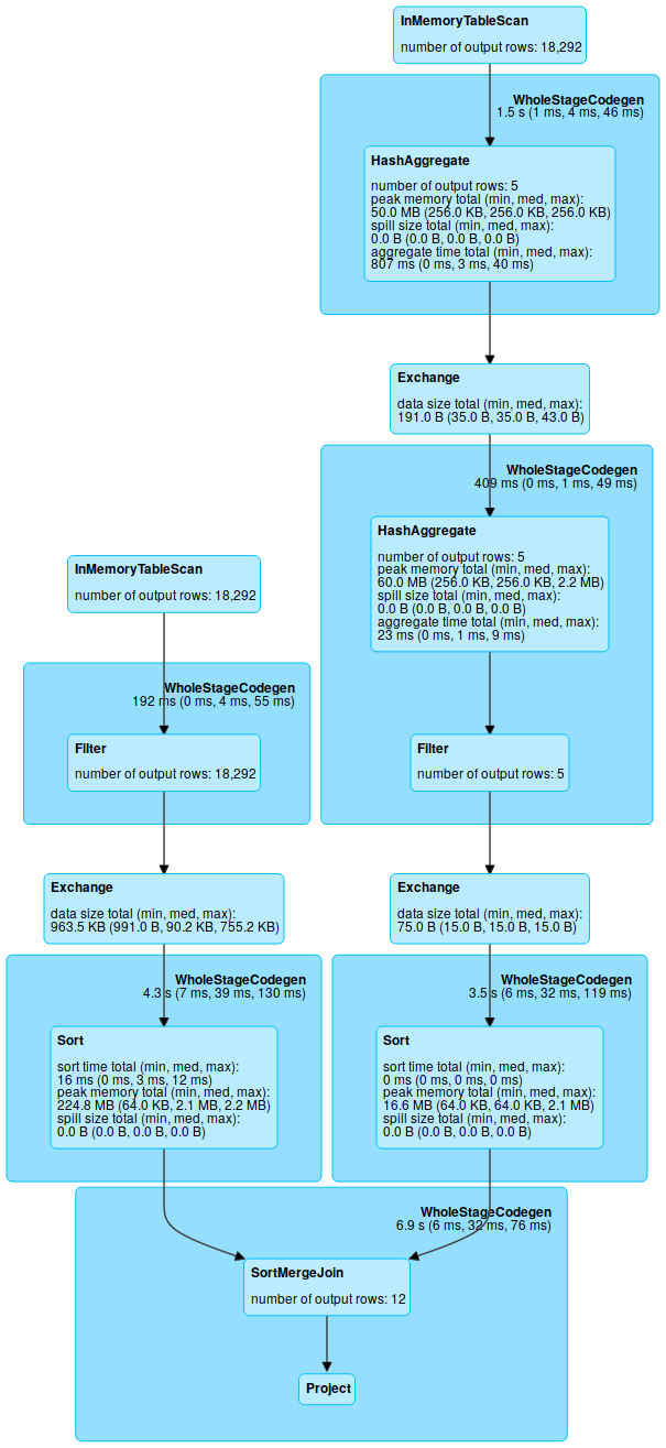
Caching
The execution plan changes, indicating that it will look in memory for that data, calculating and caching if necessary. (InMemoryRelation, InMemoryTableScan)
== Physical Plan ==
*(2) HashAggregate(keys=[mod#19L], functions=[count(1), sum(sin#21)])
+- Exchange hashpartitioning(mod#19L, 200)
   +- *(1) HashAggregate(keys=[mod#19L], functions=[partial_count(1), partial_sum(sin#21)])
      +- *(1) InMemoryTableScan [mod#19L, sin#21]
            +- InMemoryRelation [mod#19L, num_digits#20, id#17L, sin#21], StorageLevel(disk, memory, deserialized, 1 replicas)
                  +- *(1) Project [(id#17L % 3) AS mod#19L, length(cast(id#17L as string)) AS num_digits#20, id#17L, SIN(cast(id#17L as double)) AS sin#21]
                     +- *(1) Range (0, 10000, step=1, splits=6)
== Physical Plan ==
*(2) HashAggregate(keys=[mod#19L, num_digits#20], functions=[avg(id#17L), max(sin#21)])
+- Exchange hashpartitioning(mod#19L, num_digits#20, 200)
   +- *(1) HashAggregate(keys=[mod#19L, num_digits#20], functions=[partial_avg(id#17L), partial_max(sin#21)])
      +- *(1) InMemoryTableScan [mod#19L, num_digits#20, id#17L, sin#21]
            +- InMemoryRelation [mod#19L, num_digits#20, id#17L, sin#21], StorageLevel(disk, memory, deserialized, 1 replicas)
                  +- *(1) Project [(id#17L % 3) AS mod#19L, length(cast(id#17L as string)) AS num_digits#20, id#17L, SIN(cast(id#17L as double)) AS sin#21]
                     +- *(1) Range (0, 10000, step=1, splits=6)
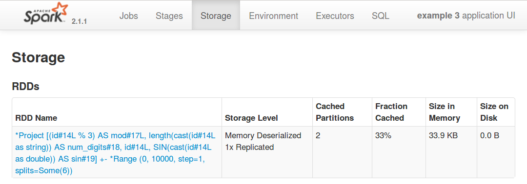
Caching
While the job is running, you can see a summary of what is currently cached in the Storage
tab of the web frontend:
Spark Optimizer
Because Spark gets the execution plan for a DataFrame all at once, it can be clever about it.
… as long as you're also clever and specify things it can work with.
Spark Optimizer
Example:
int_range = spark.range(10000000, numPartitions=6)
df1 = int_range.select(
    (int_range['id'] % 100).alias('mod'),
    functions.sin(int_range['id']).alias('sin')
)
df2 = df1.select(df1['mod'], df1['sin'] + 1)
df3 = df2.filter(df2['mod'] == 0)
df4 = df3.withColumn('mod2', df3['mod'] * 2)
df4.explain()
== Physical Plan ==
*(1) Project [(id#0L % 100) AS mod#2L, (SIN(cast(id#0L as double)) + 1.0) AS (sin + 1)#6, ((id#0L % 100) * 2) AS mod2#9L]
+- *(1) Filter ((id#0L % 100) = 0)
   +- *(1) Range (0, 10000000, step=1, splits=6)
.filter() moved before the calculation (so there's less to do); all calculations combined into one step.
Spark Optimizer
Example: never calculates the sin or sqrt because they aren't needed to generate the final result.
int_range = spark.range(10000000, numPartitions=6)
df1 = int_range.select(
    int_range['id'],
    functions.sin(int_range['id']).alias('sin'),
    functions.sqrt(int_range['id']).alias('sqrt')
)
df2 = df1.groupBy(df1['id']).count()
df2.explain()
== Physical Plan ==
*(1) HashAggregate(keys=[id#13L], functions=[count(1)])
+- *(1) HashAggregate(keys=[id#13L], functions=[partial_count(1)])
   +- *(1) Range (0, 10000000, step=1, splits=6)
Spark Optimizer
We have specified the calculations at a high-enough level that Spark can try to figure out what it really needs to do, and can do its best to get there efficiently. It's not magic, but it's pretty good.
Another example: if you spark.read a 1000-column file, it will only bring into memory the columns that are used.
Spark DAG
Another way to think of the execution plan that Spark builds which you'll see in some docs is the DAG.
You can think of the plan as a directed-acyclic graph (DAG) of DataFrames (verticies) and calculations (edges).
Spark DAG
We might draw the graph (of some fictional calculation) like this * * *

Spark DAG
If the DAG ever branches out, it's a sign that you need to .cache().

Spark DAG
The Spark web frontend will show you the DAG in the SQL
tab (broken into parts being executed as a unit, so you'll never see a branch there).
Spark Join
There is a .join() method for DataFrames: it works like a SQL join (inner join by default).
Spark Join
Some data for an example:
langs.show()
data.show()
+---+------+
| id| descr|
+---+------+
|  0| Scala|
|  1|  Java|
|  2|Python|
|  3|     R|
+---+------+
+----------+-----+---+
|      date|count| id|
+----------+-----+---+
|2022-01-01|   16|  0|
|2022-01-02|    8|  2|
|2022-01-04|   13|  0|
|2022-01-08|    4|  3|
|2022-01-15|   24|  2|
+----------+-----+---+
Spark Join
The .join method does the same as an SQL JOIN: combine data from rows that make the condition true. [The two .joins here are almost equivalent.]
joined_data = data.join(langs, on=(data['id'] == langs['id']))
joined_data = data.join(langs, on='id')
joined_data.show()
+---+----------+-----+------+
| id|      date|count| descr|
+---+----------+-----+------+
|  0|2021-01-01|   16| Scala|
|  0|2021-01-04|   13| Scala|
|  3|2021-01-08|    4|     R|
|  2|2021-01-02|    8|Python|
|  2|2021-01-15|   24|Python|
+---+----------+-----+------+
Spark Join
Let's remember this picture: our DataFrames are distributed. Think about what a .join() implies.
Spark Join
A join requires doing an all-to-all kind of movement of the data. The data from both tables needs to be rearranged so rows that make the join condition true are together.
Things will be okay with small DataFrames, but go badly if we have a lot of data.
… or so it would seem.
Spark Join
Consider this join again:
joined_data = data.join(langs, on='id')
joined_data.show()
Consider the case where langs has 4 rows (as before), but data has billions.
Spark Join
joined_data = data.join(langs, on='id')
joined_data.show()
We don't need to worry about langs as big data
. Instead, imagine it as a lookup table.
langs ≈≈ {0: ['Scala'], 1: ['Java'], 2: ['Python'], 3: ['R']}
Spark Join
langs ≈≈ {0: ['Scala'], 1: ['Java'], 2: ['Python'], 3: ['R']}
New strategy: send a copy of this to every executor (i.e. broadcast
it). Use that to produce the .join() result by just doing a lookup for every row of the larger DataFrame. That can easily be done in parallel.
Spark Join
We turned a horrible shuffle into a simple pipeline operation (projection
in relational algebra terminology) on the larger DataFrame and invented a broadcast join.
It works only if one side of the join is small enough.
Spark Join
With Spark, we can use .hint('broadcast') (or functions.broadcast()) to give a hint that the DataFrame is small enough to broadcast. The optimizer will (usually?) notice if it's about to join and a broadcast would be worthwhile.
We can see the result in the execution plan…
Spark Join
joined_data = data.join(langs, on='id')
joined_data.explain()
joined_data = data.join(langs.hint('broadcast'), on='id')
joined_data.explain()
== Physical Plan ==
*(5) Project [id#6L, date#4, count#5L, descr#1]
+- *(5) SortMergeJoin [id#6L], [id#0L], Inner
   :- *(2) Sort [id#6L ASC NULLS FIRST], false, 0
   :  +- Exchange hashpartitioning(id#6L, 200), ENSURE_REQUIREMENTS, [id=#105]
   :     +- *(1) Filter isnotnull(id#6L)
   :        +- *(1) Scan ExistingRDD[date#4,count#5L,id#6L]
   +- *(4) Sort [id#0L ASC NULLS FIRST], false, 0
      +- Exchange hashpartitioning(id#0L, 200), ENSURE_REQUIREMENTS, [id=#111]
         +- *(3) Filter isnotnull(id#0L)
            +- *(3) Scan ExistingRDD[id#0L,descr#1]

== Physical Plan ==
*(2) Project [id#6L, date#4, count#5L, descr#1]
+- *(2) BroadcastHashJoin [id#6L], [id#0L], Inner, BuildRight, false
   :- *(2) Filter isnotnull(id#6L)
   :  +- *(2) Scan ExistingRDD[date#4,count#5L,id#6L]
   +- BroadcastExchange HashedRelationBroadcastMode(List(input[0, bigint, false]),false), [id=#146]
      +- *(1) Filter isnotnull(id#0L)
         +- *(1) Scan ExistingRDD[id#0L,descr#1]
Spark Join
Join summary:
| DF 1 | DF 2 | Result |
|---|---|---|
| small | small | 😁 |
| small | big | 😁 |
| big | small | 😁 |
| big | big | 😓 * |
* but would you bet against the Spark optimizer?