More Python Techniques
More Python Techniques
Because we have a little time, let's have a look at some things you can actually do with Python.
More Python Techniques
Of course programming in general is used in many, many areas.
After learning one programming language, learning another is many times easier: the actually-hard concepts (i.e. expressing yourself in a precise-enough way for the language/computer to understand) translate to other programming languages. You have to spell your thoughts differently, but they'll be more-or-less the same thoughts.
More Python Techniques
But let's stick to Python here.
Python is a very common language for many application areas: it's commonly used so lots of help is available, it's considered nice to write, and has lots of libraries that can be installed to do useful things (e.g. Pillow).
IDEs
All semester, I (and most of you) have been using IDLE to edit Python code. The choice of IDLE was mostly because it comes with Python when you install it.
Python code is a plain text file, so it can be created/edited with any text editor. If you have/develop a preference, then you can use it.
IDEs
An IDE or Integrated Development Environment is a larger program that is a text editor integrated with programming-specific tools. IDLE is an extremely-minimal IDE.
I didn't suggest using another IDE because (1) it's another thing to install and have not work for some people, (2) they tend to be complex enough that I'd expect them to be intimidating for beginners.
IDEs
There are several good and free/semi-free IDEs for Python.
- Spyder: open source and installed with the Anaconda Python distribution.
- Visual Studio Code: free and paid versions.
- PyCharm: free student license.
IDEs
Generally IDEs offer various helpful features:
- Running code within the application.
- Highlighting errors/problems in code.
- An editor smart enough to guess when you want to indent.
- Autocomplete of functions/variables/methods that are defined in context.
- Navigation around code (e.g.
go to definition of a function
).
IDEs
If you're going to program much more, it is probably worth the investment of time to install and learn the basics of some IDE.
Type Hints
There's an optional feature in Python code we haven't been using: type hints.
Type Hints
Consider this function we wrote to reverse a string:
def reverse(s):
    if s == "":
        return ""
    else:
        return s[-1] + reverse(s[:-1])
We know the argument must be a string, and if we all it with some other type like reverse(200), it will cause an error when the program runs:
TypeError: 'int' object is not subscriptable
Type Hints
This isn't noticed until the program runs because every argument/variable can hold any type in Python. Some languages have strict requirements to declare types so they can be checked by the language before the program even starts, but Python doesn't.
Python programmers can optionally include type hints to make types of values explicit.
Type Hints
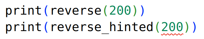
e.g. in this version of the function, it's clear that the argument must be a string, and the function returns a string.
def reverse_hinted(s: str) -> str:
    if s == "":
        return ""
    else:
        return s[-1] + reverse_hinted(s[:-1])
To give a type hint for an argument or variable, name: type
.-> type:
Type Hints
For reasons I don't understand, there's not way to make Python actually check these types: you can still call this function with an non-string argument.
Checking for mismatched types must be done with another tool, mypy. As far as I know, it's command-line only, but it will report type problems in code:
$ mypy hints.py
hints.py:15: error: Argument 1 to "reverse_hinted" has
incompatible type "int"; expected "str"  [arg-type]
Type Hints
But some IDEs can also use these type hints to
In VSCode, the setting Python > Analysis: Type Checking Mode
must be changed to Basic
or higher. (It's also a mystery to me why this isn't on by default.)
Type Hints
Then if you use a value of the wrong type somewhere, an IDE can give you a warning that something isn't right.
Mousing-over the problem gives a tooltip that explains what the IDE thinks the problem is: argument… cannot be assigned to parameter "s" of type "str"
.
Type Hints
The modules you have been given for assignments 3 and 4 are type hinted:
- with mypy config to require type hints everywhere;
- so they could be checked with mypy, eliminating any type-related mistakes that could have been hiding in the module itself;
- so any of you that happened to be using a IDE that could take advantage would get these hints;
- because it's good practice in Python.
Type Hints
You can include type hints in your code, but we won't require it.
In assignment 3, you might have started the game something like this:
hands = []  # each player's hand: list of list of Cards
banks = []  # each player's money: list of integers
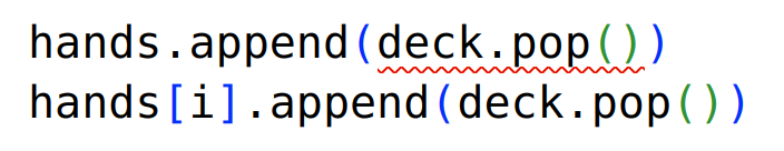
It would be easy to accidentally add a card to the hands instead of hands[i] where it belongs.
hands.append(deck.pop())
Type Hints
Type hints could be included on those variables:
hands: list[list[Card]] = []
banks: list[int] = []
An IDE now notices the problem: the thing being appended isn't the right type. It's happy with the probably-correct version (second line).
Type Hints
Is it worth including type hints? I'm not sure.
They force me to think about the type of everything, which is good. But the mistakes I make aren't usually type-related.
Your call.
Input and Output
We have really only had one way to receive data from the outside world: directly from the user with input.
Also one way to send information out: print.
It's also possible to read/write files, or read web URLs, or many other things.
Input and Output
We have seen a little of this with Pillow, which can read and write image files:
img = Image.open("picture.png")
img.save("picture.jpg")
… but it's taking care of all of the details.
Input and Output
You can open a file to read or write with the built-in open function.
This code will create two file objects: one for reading text ("rt") and one for writing text ("wt"), both using UTF-8 encoding:
infile = open(input_filename, "rt", encoding="utf-8")
outfile = open(output_filename, "wt", encoding="utf-8")
Input and Output
Reading a text file can be done by line: iterating through it with a for loop will give you one line at a time.
for line in infile:
    line_reversed = reverse(line)
    outfile.write(line_reversed)
Since we're dealing with text, each line will be a string, and we can do any string-stuff we want with it.
Input and Output
When reading/writing files as text, you are looking at them basically as a text editor does: they are made of characters which you will work with as strings in Python.
The other option is to read/write bytes: you get individual bytes from the file and you can interpret them as you like. That is generally harder, but necessary to deal with many file formats (.png, .zip, .pdf, .docx, …).
Input and Output
There are various libraries to open other file-like things.
e.g. urllib.request that you can use to open web-based resources.
Input and Output
Apparently, Pillow's Image.open can take a filename (as we have been doing), or a file object as created by open(filename, "rb") as a place to read the image from.
And urllib.request.urlopen gives us something close-enough to a file object that Pillow can read from it.
The images created for assignment 4 come from code like this…
Input and Output
from PIL import Image
from urllib.request import urlopen

IMAGES = [
    ('robot', 'https://cdn-icons-png.flaticon.com/512/3070/3070648.png'),
    ('wall', 'https://cdn-icons-png.flaticon.com/512/698/698633.png'),
    ('coin', 'https://cdn-icons-png.flaticon.com/512/1490/1490853.png'),
]

for name, url in IMAGES:
    src = urlopen(url)
    img = Image.open(src)
    img = img.resize((48, 48)).convert(mode='P', colors=8)
    img.save(name + '.png')
Input and Output
… there was a little more in the real
code than that, but not much.
The lesson: there are a lot of input/output options we haven't explored. They aren't that hard to use and can be combined fairly easily.
Jupyter Notebooks
Notebooks are a common way to experiment/interact with code. Specifically in Python, Jupyter Notebooks.
The idea: you write code in short fragments in cells
and run them piece by piece (by pressing shift-enter). Anything printed by a statement or returned by an expression is displayed below the cell.
Jupyter Notebooks
I think notebooks are a bad way to write programs: if you're writing functions, loops/if that are more than a few lines, use a text editor and write a .py file.
But if you're experimenting with data, maybe…
Data in Python
Python is also a very common language for data analysis/manipulation. It's probably the only language, unless you come from a stats background, in which case R is the other choice.
One of the most common tools to work with data in Python (but definitely not the only one) is Pandas.
Data in Python
The basic data structure in Pandas is a DataFrame that holds data as rows and columns.
Each column has a type (integer, floating point, string, date, etc) and a name (First Name
, Age
, etc). Basically the kind of data you'd commonly have in a spreadsheet.
Data in Python
Pandas is usually imported like this:
import pandas as pd
That's the same as
except renaming it to import pandaspd so you can type pd.something instead of pandas.something.
Data in Python
The, suppose we have a little DataFrame like this (we'll talk about creating them later).
     name    R    G    B
0     red  1.0  0.0  0.0
1   green  0.0  1.0  0.0
2  yellow  1.0  0.5  0.0
This is a DataFrame with four columns: name, R, G, B. The first is a string, the others are floating point. It has three rows of data, labelled 0, 1, 2.
Data in Python
Most DataFrame operations are done on a whole column at a time. It's possible to work with individual rows/cells, but uncommon and less beautiful.
Square brackets can be used to refer to a column in a DataFrame: colours["name"].
Data in Python
Operations are generally done column-at-a-time, like this:
colours["avg"] = (colours["R"] + colours["G"]
                  + colours["B"]) / 3
The calculations are all done element-by-element: that's each red, plus the corresponding green, plus the blue, all divided by three
.
Data in Python
Let's try another calculation: relative luminance, which (if I'm reading the Wikipedia page correctly) is this, and sort:
colours["luminance"] = (0.2126 * colours["R"]**2.2
                        + 0.7152 * colours["G"]**2.2
                        + 0.0733 * colours["B"]**2.2)
colours.sort_values("luminance", inplace=True)
After this, the DataFrame is:
     name    R    G    B       avg  luminance
0     red  1.0  0.0  0.0  0.333333   0.212600
2  yellow  1.0  0.5  0.0  0.500000   0.368254
1   green  0.0  1.0  0.0  0.333333   0.715200
Data in Python
Often when working in Pandas (and other big frameworks
for various problem domains), almost every line of code is some interaction with the library.
It can start to feel like you're not writing Python
anymore, but mostly writing Pandas
code.
Data in Python
Rather than trying to give a comprehensive tour of a huge toolkit, I'm going to work through an example data set, as I might have explored it using Pandas and related tools.
I'll experiment with the GeoNames cities >1000 people data.
Data in Python
I'm going to start with the data as exported from opendatasoft rather than the original cities1000.txt: it's in a more common format, so the DataFrame is created in a more typical way.
That data is in CSV format with a header row (i.e. if loaded into a spreadsheet, row 1 would be column names and the rest is data), except with semicolons instead of commas.
Data in Python
Pandas can read a CSV file into a DataFrame. There are many options, but most of the defaults line up with the usual way CSV files are formatted, including having a header row.
cities = pd.read_csv("geonames-all-cities-with-a-population-1000.csv",
                     sep=";")
Data in Python
That line gets us a fun data set:
        Geoname ID          Name  ... LABEL EN         Coordinates
0          2844437     Rotenburg  ...  Germany   53.11125, 9.41082
1          2845209    Ronshausen  ...  Germany         50.95, 9.85
2          2845304       Römhild  ...  Germany  50.39639, 10.53889
3          2845721      Rohrbach  ...  Germany  48.61667, 11.56667
4          2845747          Rohr  ...  Germany  49.34112, 10.88981
...            ...           ...  ...      ...                 ...
147038     2667499  Träslövsläge  ...   Sweden  57.05417, 12.27899
147039     2673829     Stigtomta  ...   Sweden      58.8, 16.78333
147040     2674649  Staffanstorp  ...   Sweden  55.64277, 13.20638
147041     2682706        Resarö  ...   Sweden   59.4291, 18.33386
147042     2686674       Örbyhus  ...   Sweden  60.22407, 17.70138

[147043 rows x 20 columns]
Data in Python
We can extract a few columns if we want to have a closer look (with square brackets containing a list of column names):
print(cities[["Name", "Population", "Coordinates"]])
                Name  Population         Coordinates
0          Rotenburg       22139   53.11125, 9.41082
1         Ronshausen        2409         50.95, 9.85
2            Römhild        1888  50.39639, 10.53889
3           Rohrbach        6015  48.61667, 11.56667
4               Rohr        3372  49.34112, 10.88981
...              ...         ...                 ...
Data in Python
Let's check the most populous cities in the data set:
largest = cities.sort_values("Population", ascending=False)
print(largest[["Name", "Population"]].iloc[:10])
             Name  Population
95066    Shanghai    22315474
61505     Beijing    18960744
35685    Shenzhen    17494398
103721  Guangzhou    16096724
73164    Kinshasa    16000000
136986      Lagos    15388000
71815    Istanbul    14804116
143552    Chengdu    13568357
38307      Mumbai    12691836
124135  São Paulo    12400232
Data in Python
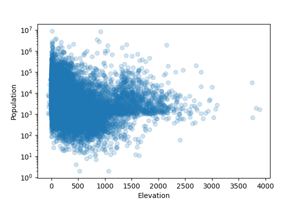
Let's have a look at a quick visualization to see what's going on. The Matplotlib library is the most commonly used plotting library for Python.
import matplotlib.pyplot as plt
fig, ax = plt.subplots(figsize=(6, 4))
ax.scatter(cities['Elevation'], cities['Population'], alpha=0.2)
ax.set_xlabel('Elevation')
ax.set_ylabel('Population')
ax.set_yscale('log')
fig.savefig("ele-pop.png")
Data in Python
We can see a little more of what's happening:
Data in Python
Hmm… this is supposed to be cities >1000 people
data, but there are a bunch of places with population <1000 in there.
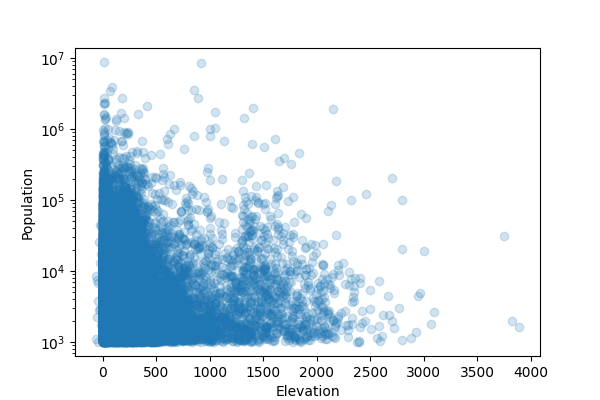
I'm suspicious of those entries: let's remove them from the data set. The […] can also be given a boolean filter: rows where it evaluates to True are kept.
cities = cities[cities["Population"] >= 1000]
Data in Python
Now it looks more like I would expect:
Data in Python
How do average city
sizes compare? Let's look at the average for a few countries:
na_cities = cities[
    cities["Country Code"].isin(["CA", "US", "MX"]) ]
avg_pop = na_cities.groupby("Country Code") \
        .agg({"Population": "mean"})
print(avg_pop)
                Population
Country Code
CA            27632.266055
MX            12867.040948
US            16378.814702
Data in Python
avg_pop = na_cities.groupby("Country Code") \
        .agg({"Population": "mean"})
A group by
operation involves combining the groups of rows that have the same value (the same country code here). Then those group are aggregated by doing some calculation on some/all other columns: mean, min, max, count, sum, etc.
Data in Python
I'm surprised how different the averages are. It seems like Canada might have fewer small towns
, likely because of the way we arrange municipalities rather than where we live.
Is there a signficant difference between the sizes of Canadian and US cities?
Data in Python
The SciPy library contains implementations of several statistical tests (as well as numeric integration, signal processing, liear algebra, …). The statsmodels library has more.
Data in Python
Mann-Whitney seems like a reasonable test for this situation. We can give it the city populations from Canada and the USA.
from scipy.stats import mannwhitneyu
canada = cities[cities["Country Code"] == "CA"]
usa = cities[cities["Country Code"] == "US"]
u = mannwhitneyu(canada["Population"], usa["Population"])
print(u.pvalue)
2.5605149325211987e-09
The
is e-09\(\mbox{}\times 10^{-9}\)
, so that's a very small p-value. We reject the null and conclude there's something different about the populations.
Data in Python
What about within Canada? Do the provinces have different city sizes?
There's no obvious indication of the province each city is in, but the data has a column Admin1 Code
.
The admin1CodesASCII.txt from GeoNames contains the answer: it will tell us that CA.02
actually means British Columbia
.
Data in Python
It's tab-separated and doesn't contain a header row. We can still read it into a DataFrame:
ac_names = ["code", "Admin Name", "Admin Name ascii",
            "Admin geonameid"]
admin_codes = pd.read_csv("admin1CodesASCII.txt", sep="\t",
                          names=ac_names)
admin_codes = admin_codes[["code", "Admin Name"]]
Data in Python
print(admin_codes[admin_codes["code"].str.startswith("CA")])
      code                 Admin Name
466  CA.01                    Alberta
467  CA.02           British Columbia
468  CA.03                   Manitoba
469  CA.04              New Brunswick
470  CA.13      Northwest Territories
471  CA.07                Nova Scotia
472  CA.14                    Nunavut
473  CA.08                    Ontario
474  CA.09       Prince Edward Island
475  CA.10                     Quebec
476  CA.11               Saskatchewan
477  CA.12                      Yukon
478  CA.05  Newfoundland and Labrador
Data in Python
We can then join those two together: get cities from CA.02
together with the string British Columbia
.
But the original data doesn't have CA.02
in it: it has a column Country Code
and another Admin1 Code
that contain those two things separately. But we can build it and then use the equal values as the basis to join the two data sets.
Data in Python
cities["code"] = cities["Country Code"] + "." \
                 + cities["Admin1 Code"]
merged = pd.merge(cities, admin_codes, on="code")
canada = merged[merged["Country Code"] == "CA"]
print(canada[["Name", "code", "Admin Name"]])
                   Name   code             Admin Name
49035        Ballantrae  CA.08                Ontario
49036   Bayview Village  CA.08                Ontario
49037         Brantford  CA.08                Ontario
49038         Fort Erie  CA.08                Ontario
49039      Fort Frances  CA.08                Ontario
...                 ...    ...                    ...
121835      Yellowknife  CA.13  Northwest Territories
121836        Behchokǫ̀  CA.13  Northwest Territories
121837        Hay River  CA.13  Northwest Territories
121838           Inuvik  CA.13  Northwest Territories
121839     Norman Wells  CA.13  Northwest Territories
Data in Python
Then we can to the same statistical test on a couple of provinces and see if we find anything.
ns = canada[canada["Admin Name"] == "Nova Scotia"]
qc = canada[canada["Admin Name"] == "Quebec"]
u = mannwhitneyu(ns['Population'], qc['Population'])
print(u.pvalue)
0.39906900974160187
Nope: \(p ≥ 0.05\) so we can draw no conclusion.
Data in Python
Or maybe we should rephrase it as a categorical question. For a chi-squared (\(\chi^2\)) test, we need a contingency table
: a count of how many items are in each category pair.
I'll look at big
cities and see if their frequency varies by country.
na_cities["is_big"] = na_cities["Population"] > 20000
Data in Python
Pandas' crosstab function is exactly what we need to build a contingency table.
counts = pd.crosstab(na_cities["Country Code"],
                     na_cities["is_big"])
print(counts)
is_big        False  True
Country Code
CA              945    254
MX             8195    499
US            13818   2534
i.e. there are 945 Canadian cities with population ≤20000 and 254 with population >20000.
Data in Python
Then a chi-squared test is a function call away:
from scipy.stats import chi2_contingency
print(chi2_contingency(counts).pvalue)
1.668349751262136e-126
So, we reject the null and conclude there's some relationship between (North American) country and big/small cities.
Data in Python
As basic data analysis goes, this cities data was relatively technically demanding: non-standard CSV format, multiple DataFrames to be joined on values that had to be computed.
Taking already-nice data (e.g. a single .csv file saved from Excel or Sheets) and doing basic manipluation on it can be just a few lines of code.
More Python Data Tools
There is a massive collection of data manipulation tools for Python. Mentioned here: Pandas, matplotlib, SciPy, statsmodels.
What was mentioned here was just the tiniest overview of what's in them. Learning all of them is hopeless. Learning a few core tools/techniques and getting an idea of what else is out there (and being willing to read the docs) is totally achievable if you want/need them.
More Python Data Tools
There are also other Python DataFrame tools: Polars which promises to be more modern and faster, and Spark for big data (≈ >1 computer needed to store/compute).
Advice: look at them if your data set is too big to comfortably work with in Pandas. Otherwise, stay with the more-online-help world of Pandas.
More Python Data Tools
Other plotting libraries: Seaborn that extends/enhances matplotlib, and Plotly for interactive graphs.
Perhaps also of interest: The Python Graph Gallery, a collection of data visualization techniques and Python code to generate them.
More Python Data Tools
- SymPy: symbolic mathematics and algebraic manipulation.
- scipy.linalg: linear algebra tools (inverting matrices, solving linear equations, etc).
- RDKit: a toolkit for cheminformatics.
- Pygame for game development.
- Python will be supported in Excel, but it still in
preview
.
Summary
None of the topics from this slide deck will be on the final exam.